This is the second part of “An Outsider’s Tour of Reinforcement Learning.” Part 3 is here. Part 1 is here.
In addition to the reasons I’ve discussed so far, I’ve been fascinated with the resurgence in reinforcement learning because it operates at the intersection of two areas I love: machine learning and control. It is amazing how little we understand about this intersection. And the approaches used by the two disciplines are also frequently at odds. Controls is the theory of designing complex actions from well-specified models, while machine learning makes intricate, model-free predictions from data alone.
At the core of control theory are dynamical systems with inputs and outputs. These systems have internal state which reacts to current conditions and the inputs, and the outputs are some function of the state and the input. If we are to turn off the inputs, the state is all we need to know to predict the future output for all time.
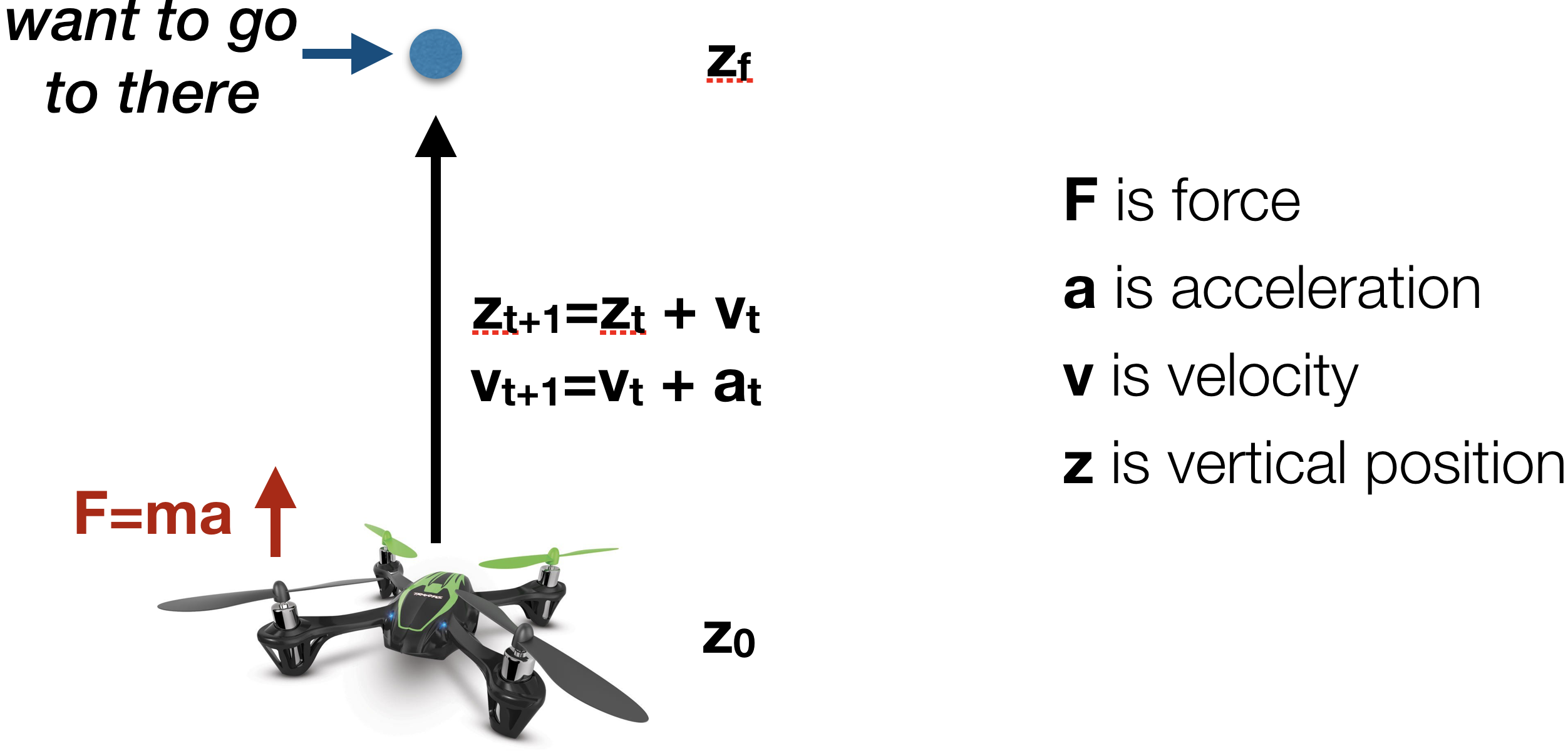
As a simple example, remember Newton’s laws. Say that we want to fly a quadrotor floating at 1 meter off the ground to 2 meters off the ground. In order to raise the position, we’d increase the propeller speed to create an upward force. Propeller speed is an input. The force must be strong enough to counteract gravity which can be considered another input. The dynamics then follow Newton’s laws: the acceleration is proportional to the total force applied minus gravity. It is inversely proportional to the mass of quadrotor. The velocity is equal to the previous velocity plus some multiple of acceleration. And the position is equal to the previous position plus a multiple of velocity. From these equations we can compute a set of forces that lift the quadrotor up to the desired height. The state of the system here is pair of position and velocity.
I can write such a dynamical system compactly as a difference equation
\[x_{t+1} = f(x_t, u_t, e_t)\]Here $f$ is a deterministic function that tells us what the next state will be given the current state, the current input, and an error signal $e_t$. $e_t$ could be random noise in the system or a systematic error in the model. For simplicity, let’s assume for now that the $e_t$ is random.
Optimal control asks to find a set of inputs that minimizes some objective. We assume that at every time, we receive some reward for our current $x_t$ and $u_t$ and we want to maximize this reward. In math terms, we aim to solve the optimization problem
\[\begin{array}{ll} \mbox{maximize} & \mathbb{E}_{e_t}[ \sum_{t=0}^N R_t[x_t,u_t] ]\\ \mbox{subject to} & x_{t+1} = f(x_t, u_t, e_t) \end{array}\]That is, we aim to maximize the expected reward over $N$ time steps with respect to the control sequence $u_t$, subject to the dynamics specified by the state transition rule $f$. If you are an optimization person, you are now ready to be a controls engineer: model your problem into an optimal control problem and then call your favorite solver. Problem solved! This sounds like I’m joking, but there is a large set of control problems that are solved in precisely such a manner. And one of the earliest algorithms devised to solve them was back propagation.
Another important example of $f$ is that of a Markov Decision Process (MDP). Here $x_t$ takes on discrete values. $u_t$ is a discrete control action. $x_t$ and $u_t$ together determine the probability distribution of $x_{t+1}$. In MDP, everything can be written out as probability tables, and the problem can be solved via dynamic programming.
Now let’s bring learning into this picture. What happens when we don’t know $f$? In our quadrotor example, we might not know the force output by our propellers given a control voltage. Or we could have something considerably more complicated: we might have a massive data center with complex heat transfer interactions between the servers and the cooling systems.
There are a couple of obvious things you might try here. First, you can fit a dynamics model after running experiments to explore what the system is capable of under different input settings. Then you can use this model inside an optimal control problem. For some systems, this is a reasonable approach: for a quadrotor there are usually only a few parameters needed for actual control, and these can be estimated individually from simple calibration experiments.
For more complicated systems, it might be hard to even write out a parametric model in closed form. In this case, an alternative approach is to disregard models altogether and to just try to increase the reward based on measurement of the state $x_t$. This approach would closely align with the “prescriptive analytics” characterization of reinforcement learning that I described in my previous post. Such an prescriptive approach would not only be useful for creating controls from scratch, but could also be helpful if the model somehow changes over time due to some sort of unmodeled drift. But also note that this purely reactive approach to control disregards crucial information about time-dependencies in the inference task and also demands that you disregard 400 years of enlightenment physics in your control design plan.
The key questions for evaluating these different approaches are: how well must we understand and model a dynamical system in order to control it optimally? What is the optimal way to query and probe a system to achieve high quality control with as few interventions as possible?
These questions form the core of the classical core problems of reinforcement learning. And to my surprise in working through the results in this space, very little is known about how many samples are needed and which methods are more or less efficient. In these next few blogs I’ll try to establish some baselines that highlight the pros and cons of these various approaches to optimal control with unknown dynamics.