A common sticking point in contemporary reinforcement learning is how to evaluate performance on benchmarks. For a general purpose method, we’d like to demonstrate aptitude on a wide selection of test problems with minimal special case tuning. A great example of such a suite of test problem is the Arcade Learning Environment (ALE) of Atari benchmarks. How can we tell when an algorithm is “state-of-the-art” on Atari? Clearly, we can’t just excel on one game. There are 60 games, and even careful comparisons end in impenetrable tables with 60 rows and multiple columns. Moreover, the performance is a random variable as the methods are evaluated over many random seeds, so there are inherent uncertainties in the reported numbers. How can we summarize the performance over such a large number of noisy benchmarks?

Performance Profiles

My favorite way to aggregate benchmarks was proposed by Dolan and More and called performance profiles. The idea here is very simple. We want a way of depicting how frequently is a particular method within some distance of the best method for a particular problem instance. To do so, we make statistics. Let’s suppose we have a suite of $n_p$ problem instances and we want to find the best performing method across all of these instances.

For each problem instance, we compute the best method, and then for every other method, we determine how far they are from optimal. This requires some notion of “far from optimality.” Let’s denote $d[m,p]$ the distance from optimality of method m on problem p. We then count on how many problem instances a particular method is within a factor of tau of the optimal. That is, we compute

That is, we compute the fraction of problems where method m has distance from optimality less than tau.

A performance profile plots $\rho_m(\tau)$ for each method m. Performance profiles provide a visually striking way to immediately eyeball differences in performance between a set of candidate methods over a suite of benchmarks. They let you easily read off the percentage of times a method is within some set range of optimal across the suite of benchmarks. Moreover, they have several nice properties: performance profiles are robust to outlier problems. They are also robust to small changes in performance across all problems. Performance profiles allow a holistic view of performance without having to single out the idiosyncrasies of particular instances.

The canonical application for performance profiles is for comparing solve times of different optimization methods. In this case, distance from optimality will be the ratio of the time a solver takes to the time taken by the fastest on a particular instance. The original Dolan and More paper has several examples showing that performance profiles cleanly delineate aggregate differences in run times for different solvers. They are now a widely adopted convention for comparing optimization methods. As we will now see, performance profiles also provide a straightforward way to compare relative rewards in reinforcement learning problems.

Is Deep RL better than handcrafted representations on Atari?

Let’s apply performance profiles to understand the power of deep reinforcement learning on Atari games. One of my favorite deep reinforcement learning papers is “Revisiting the Arcade Learning Environment: Evaluation Protocols and Open Problems for General Agents” by Machado et al. which proposes several guidelines for conducting careful evaluations of methods on the ALE benchmark suite. When put on the same footing under their evaluation framework, DQN doesn’t look to be that much better than SARSA (a simple method for Q-learning with function approximation) and hand crafted features.

Nonetheless, the authors concede that “Despite this high sample complexity, DQN and DQN-like approaches remain the best performing methods overall when compared to simple, hand-coded representations.” But it’s hard to tell how much better DQN is. The evaluations are stochastic, and since DQN is costly, they only evaluate it’s performance on 5 random seeds and report the mean and standard deviation.

I downloaded the source of the Machado paper and parsed the results tables into a CSV file¹. This table lists the mean reward and standard deviation for each game evaluated. Not only are the rewards here random variables, but directly comparing the means is difficult because the rewards are all on completely different scales.

To attempt to address both the stochasticity and the varied scaling of of the rewards, I decided to use p-values from the Welsh t-test. That is $d[m,p]$ is the negative log probability that method $m$ has a higher score than the best method on problem $p$ under the assumptions of the Welch t-test. For the best performing method, I assign $d[m,p]=0$.

Now, this is a very imperfect measure. T-tests are assuming Gaussian distributions, and that’s clearly not going to be legitimate. But it’s not a terrible comparison when we are only provided means and variances. And, frankly, the community might want to consider releasing more finely detailed reports of their experiments if they would like better evaluation of the relative merits of methods. For example, if researchers simply released the raw scores for all runs, we could try more sophisticated nonparametric rank tests.

Let’s leave the imperfection aside for a moment, and plot a performance profile based on these likelihoods.I computed a standard performance profile for the ALE benchmark suite, plotting the frequency of the time that the p-values are greater than some threshold $\tau$. The results are here:

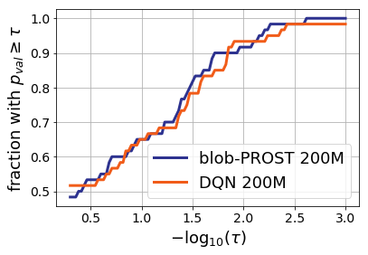
For any $x$ value, the $y$-value is the number of instances where a method either has the highest mean or where we cannot reject the null hypothesis that the method has the highest mean with confidence $\tau$. You might look at this plot and think “that’s completely unreadable as the curves are on top of each other.” When performance profiles intersect each other multiple times, it means the algorithms are effectively equivalent to each other: there is no value of $\tau$ where DQN or Blob-PROST are more frequently scoring higher than the other. To see an example of curves where things are way off, consider Blob-Prost with 200M simulations vs DQN with 10M simulations:

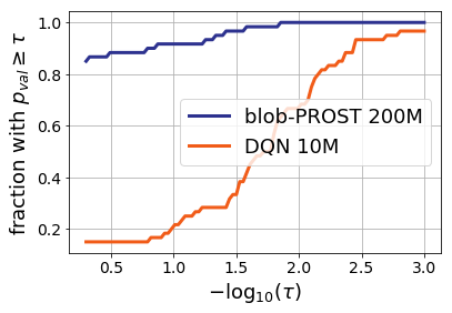
Now there is a clear separation in the performance profiles, and it’s clear that BlobProst 200M is much better than DQN 10M. This shouldn’t be surprising as I’m letting BlobProst see 20x as many samples. But it does suggest that DQN and Blob-PROST when given the same sample allocation are essentially indistinguishable methods. My take away from this plot is that Machado et al. concede too much in their discussion: simple methods and hand crafted features match the performance of DQN on the ALE.

To establish dominance, provide more evidence.

Miles Brundage suggests that there are far better baselines now (from the DeepMind folks). I’d like to make the modest suggestion that someone at DeepMind adopt the Machado et al. evaluation protocol for these new, more sophisticated methods, and then report means and standard deviations on all of the games. Even better, why not report the actual values over the runs so we could use non-parametric test statistics? Or even better, why not release the code? I’d be happy to make a performance profile again so we can see how much we’re improving.

If you are interested in changing the performance metric or running performance profiles on your own data, here’s a Jupyter notebook. that lets you recreate the above plots.