This is the tenth part of “An Outsider’s Tour of Reinforcement Learning.” Part 11 is here. Part 9 is here. Part 1 is here.
Though I’ve spent the last few posts casting shade at model-free methods for reinforcement learning, I am not blindly against the model-free paradigm. In fact, the most popular methods in core control systems are model free! The most ubiquitous control scheme out there is PID control, and PID has only three parameters. I’d like to use this post to briefly describe PID control, explain how it is closely connected to many of the most popular methods in machine learning, and then turn to explain what PID brings to the table over the model-free methods that drive contemporary RL research.
PID in a nutshell
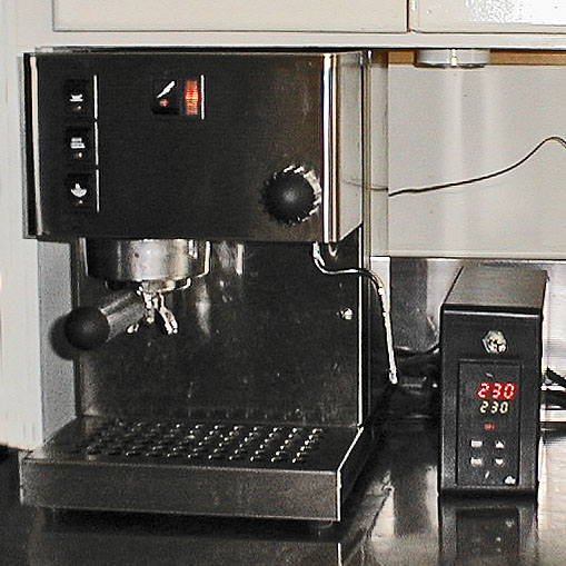
PID stands for “proportional integral derivative” control. The idea behind PID control is pretty simple: suppose you have some dynamical system with a single input that produces a single output. In controls, we call the system we’d like to control the plant, a term that comes from chemical process engineering. Let’s say you’d like the output of your plant to read some constant value $y_t = v$. For instance, you’d like to keep the water temperature in your espresso machine at precisely 203 degrees Fahrenheit, but you don’t have a precise differential equation modeling your entire kitchen. PID control works by creating a control signal based on the error $e_t=v-y_t$. As the name implies, the control signal is a combination of error, its derivative, and its integral:
\[u_t = k_P e_t + k_I \int_0^t e_s ds + k_D \dot{e}_t\,.\]I’ve heard differing accounts, but somewhere in the neighborhood of 95 percent of all control systems are PID. And some suggest that the number of people using the “D” term is negligible. Something like 95 percent of the myriad collection of control processes that keep our modern society running are configured by setting two parameters. This includes those third wave espresso machines that fuel so much great research.
In some sense, PID control is the “gradient descent” of control: it solves most problems and fancier methods are only needed for special cases. The odd thing about statistics and ML research these days is that everyone knows about gradient descent, but almost none of the ML researchers I’ve spoken to know anything about PID control. So perhaps to explain the ubiquity of PID control to the ML crowd, it might be useful to establish some connections to gradient descent.
PID in discrete time
Before we proceed, let’s first make the PID controller digital. We all design their controllers in discrete time rather than continuous time since we do things on computers. How can we discretize the PID controller? First, we can compute the integral term with a running sum:
\[w_{t+1} = w_t + e_t\]When $w_0=0$, then $w_t$ is the sum of the sequence $e_s$ for $s<t$.
The derivative term can be approximated by finite differences. But since taking derivatives can amplify noise, most practical PID controllers actually filter the derivative term to damp this noise. A simple way to filter the noise is to let the derivative term be a running average:
\[v_{t} = \beta v_{t-1} + (1-\beta)(e_t-e_{t-1})\,.\]Putting everything together, a PID controller in discrete time will take the form
\[u_t = k_P e_t + k_I w_t + k_D v_t\]Integral Control
Let’s now look at pure integral control. We can simplify the controller in this case to one simple update formula:
\[u_t = u_{t-1}+k_i e_t\,.\]This should look very familiar to all of my ML friends out there as it looks an awful lot like gradient descent. To make the connection crisp, suppose that the plant we’re trying to control takes an input $u$ and then spits out the output $y= f’(u)$ for some fixed function $f$. If we want to drive $y_t$ to zero, then the error signal $e$ takes the form $e = -f’(u)$. With this model of the plant, integral control is gradient descent. Just like in gradient descent, integral control can never give you the wrong answer. If you converge to a constant value of the control parameter, then the error must be zero.
Proportional Integral Control
As discussed above, PI control is the most ubiquitous form of control. For optimization, it is less common, but still finds a valid algorithm when $e = -f’(u)$.
Doing a variable substitution, the $PI$ controller will take the form
\[u_{t+1} = u_t + (k_I-k_P) e_t + k_P e_{t+1}\]If $e_t = -f’(u_t)$, then we get the algorithm:
\[u_{t+1} + k_P f'(u_{t+1}) = u_t - (k_I-k_P) f'(u_t)\]This looks a bit tricky as somehow we need to compute the gradient of $f$ at our current time step. However, optimization friends out there will note that this equation is the optimality conditions for the algorithm
\[u_{t+1} = \mathrm{prox}_{k_P f} ( u_t - (k_I-k_P) f'(u_t) )\,.\]Hence, PI control combines a gradient step with a proximal step. The algorithm is a hybrid between the classical proximal point method and gradient descent. Note that if this method converges, it will again converge to a point where $f’(u)=0$.
Proportional Integral Derivative Control
The master algorithm is PID. What happens here? Allow me to do a clever change of variables that Laurent Lessard showed to me. Define the auxiliary variable
\[x_t = \frac{1}{1-\beta}w_t+\frac{\beta}{(1-\beta)^3}v_t-\frac{\beta}{(1-\beta)^2}e_t\,.\]In terms of this new hidden state, $x_t$, the PID controller reduces to the tidy set of equations:
\[\begin{aligned} x_{t+1} &= (1+\beta)x_t -\beta x_{t-1} + e_t\\ u_t &= C_1 x_t + C_2 x_{t-1}+ C_3 e_t\,, \end{aligned}\]and the coefficients $C_i$ are given by the formulae:
\[\begin{aligned} C_1 &= -(1-\beta)^2 k_D+k_I\\ C_2 &= (1-\beta)^2 k_D-\beta k_I\\ C_3 &= k_P + (1-\beta) k_D \end{aligned}\]The $x_{t}$ sequence looks like a momentum sequence used in optimization. Indeed, with proper settings of the gains, we can recover a variety of algorithms that we commonly use in machine learning. Gradient descent with momentum with learning rate $\alpha$—-also known as the Heavy Ball method—is realized with the settings.
\[k_I = \frac{\alpha}{1-\beta}\,, ~~~~ k_D=\frac{\alpha \beta}{(1-\beta)^3} \,, ~~~~ k_P = \frac{-\alpha \beta}{(1-\beta)^2}\]Nesterov’s accelerated method pops out when we set
\[k_I = \frac{\alpha}{1-\beta} ~~~~ k_D=\frac{\alpha \beta^2}{(1-\beta)^3}~~~~ k_P = \frac{-\alpha \beta^2}{(1-\beta)^2}\]These are remarkably similar, differing only in the power of $\beta$ in the numerator of the proportional and derivative terms.
The Lur’e Problem
Laurent blew my mind when he showed me the connection between PID control and optimization algorithms. How crazy is it that most of the popular algorithms in ML end up being special cases of PID control? And I imagine that if we went out and did surveys of industrial machine learning, we’d find that 95% of the machine learning models in production were trained using some sort of gradient descent. Hence, there’s yet another feather in the cap for PID.
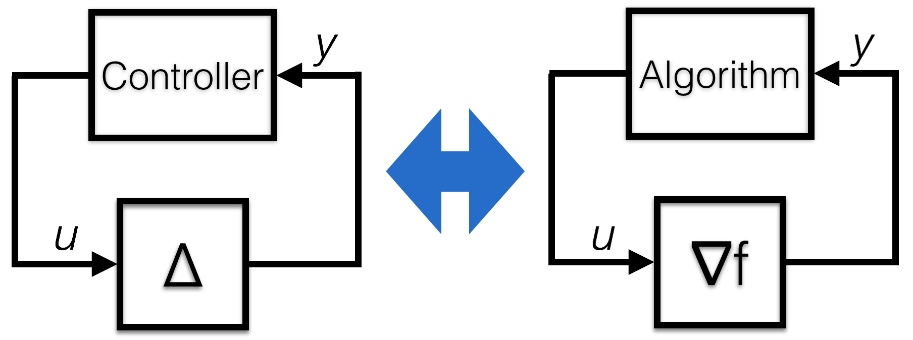
It turns out that the problem of feedback with a static, nonlinear map has a long history in controls, and this problem even has a special name: the Lur’e problem. Finding a controller to push a static nonlinear system to a fixed point turns out to be identical to designing an optimization algorithm to set a gradient to zero.
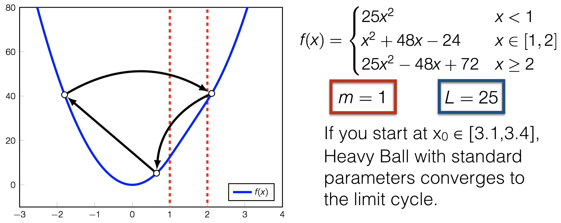
Laurent Lessard, Andy Packard, and I made these connections in our paper, showing that many of the rates of convergence for optimization algorithms could be derived using stability techniques from controls. We also used this approach to show that the Heavy Ball method might not always converge at an accelerated rate, justifying why we need the slightly more complicated Nesterov accelerated method for reliable performance. Indeed, we found settings where the Heavy Ball method for quadratics converged linearly, but on general convex functions didn’t converge at all. Even though these methods barely differ from each other in terms of how you set the parameters, this subtle change is the difference between convergence and oscillation!
With Robert Nishihara and Mike Jordan, we followed up this work showing that you could even use this to study ADMM using the connections between prox-methods and proportional integral control. Bin Hu, Pete Seiler, and Anders Rantzer generalized this technique to better understand stochastic optimization methods. And Laurent and Bin made the formal connections to PID control that I discuss in this post.
Learning to learn
With the connection to PID control in mind, we can think of learning rate tuning as controller tuning. The Nichols-Ziegler rules (developed in the forties) simply find the largest gain $k_P$ such that the system oscillates, and set the PID parameters based on this gain and the frequency of the oscillations. A common trick for gradient descent tuning is to find the largest value such that gradient descent does not diverge, and then set the momentum and learning rate accordingly from this starting point.
Similarly, we can think of the “learning to learn” paradigm in machine learning as a special case of controller design. Though PID works for most applications, it’s possible that a more complex controller will work for a particular application. In the same vein, it’s always possible that there’s something better than Nesterov’s method if you restrict your set of instances. And maybe you can even find this controller by gradient descent. But it’s always good to remember, 95% is still PID.
I make these connections for the following reason: both in the case of gradient descent and PID control, we can only prove reasonable behavior in rather constrained settings: in PID we understand how to analyze certain nonlinear control systems, but not all of them. In optimization, we understand the behavior on convex functions and problems that are “nearly” convex. Obviously, we can’t hope to have simple methods to stabilize all possible plants/functions (or else we’re violating some serious conjectures in complexity theory), but we can show that our methods work on simple cases, and performance degrades gracefully as we add complexity to the problem.
Moreover, the simple cases give us a body of techniques for general design: by developing theory on specific cases we can developing intuition and probe fundamental limits. I think the same thing needs to be established for general reinforcement learning, and it’s why I’ve been spending so much time on LQR and nearby generalizations.
Let’s take this perspective for PID. Though PID is a powerful workhorse, it is typically thought of to only be useful for simple low-level control loops attempting to maintain some static equilibrium. It seems like it’s not particularly useful for more complex tasks like robotic acrobatics. However, in the next post, I will describe a more complex control task that can also be solved by PID-type techniques.