A massive cluster-randomized controlled trial run in Bangladesh to test the efficacy of mask wearing on reducing coronavirus transmission released its initial results and the covid pundits have been buzzing with excitement. There have already been too many hot takes on the report, but, after wrangling with the 94 pages, I came to a different conclusion than most who have used this study as evidence for their mask predilections. I worry that because of statistical ambiguity, there’s not much that can be deduced at all.
The Bangladesh mask study was a cluster-randomized controlled trial. Rather than randomizing patients, this study randomized villages. Though the sample size looked enormous (340,000 individuals), the effective number of samples was only 600 because the treatment was applied to individual villages. Villages were paired using demographic attributes and one of each pair was randomly assigned to an intervention and the other to no intervention. The 300 intervention villages received free masks, information on the importance of masking, role modeling by community leaders, and in-person reminders for 8 weeks. The 300 villages in the control group did not receive any interventions.
The goal was to determine how much these interventions contributed to patients who both reported symptoms, subsequently consented to antibody testing, and tested positive. The study reports the precise number of people who report symptoms down to the single person (13,273 in treatment, 13,893 in control). The study reports the precise number of symptomatic people who consented to blood draws (5,414 in treatment, 5,538 in control). And the study reports the precise number of blood draws that were tested for covid antibodies (5,006 in treatment, 4,971 in control). But here’s where the picture gets murky: The number of actual positive tests appears nowhere in the preprint.
The study reports that 0.76% of the people in the control villages were symptomatic and seropositive whereas 0.69% of the people in the treatment villages were symptomatic and seropositive. This corresponds to about a 1.1 fold reduction in risk, and this result was deemed by the authors to be statistically significant.
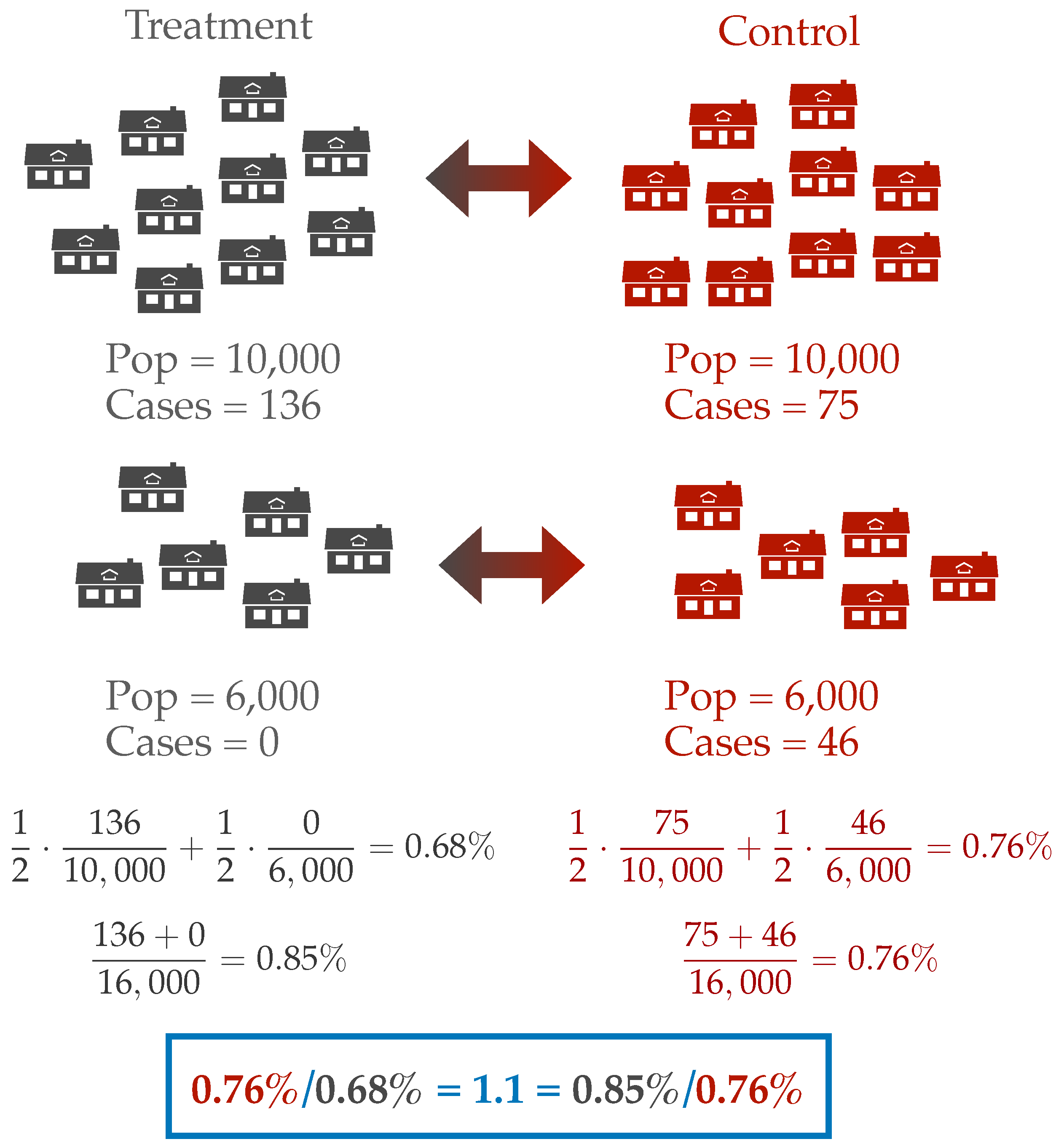
Where do these seropositivity percentages come from? The paper does not make clear what is being counted. Do the authors compute the number of cases in treatment divided by the number of individuals treated? Or do they compute the prevalence in each cluster and average these up? These two different estimates of prevalence can give different answers. For instance, we can imagine a simplified scenario with two clusters. Let’s say one treatment-control pair consists of two villages with 10,000 people each and pair two consists of villages with 6,000 people. In the larger treatment village, there is an outbreak with 136 cases, but in the smaller treatment village there are no cases. In the control villages, the larger village observes 75 cases and the smaller 46 cases. If we count over the number of individuals, then the prevalence ratio is 1.1 in favor of the control arm. However, if we first compute prevalence at the village level and then average these estimates, we find a prevalence ratio of 1.1 in favor of the treatment arm. But which is better? Reducing prevalence at the village level or the population level? This question is especially difficult when the actual magnitude of the outcome is so small. In either case we are talking about a difference of 15 cases between the treatment and control villages in a population of 32,000 individuals.
When effect sizes are small and sensitive to measurement, convention compels us to find refuge in an argument over statistical significance. So let’s then examine how significance is derived in the working paper. The authors say that they model the count of symptomatic seropositive individuals as a “a generalized linear model (GLM) with a normal family and identity link.” This is a fancy way of saying that they modeled the count as if it were sampled from a normal distribution and ran ordinary least-squares regression. Based on the captions on the tables, it appears that they modeled the rate of symptomatic seroprevalence in each village as a normal distribution whose mean is a function of the village cluster and some other covariates. They then apparently computed estimates of village level seroprevalence under the model and averaged these estimates to yield a final estimate of seroprevalence in treatment and control.
While the Gaussian model made the authors’ coding simple and allowed them to report results in standard econometric formatting, the model is also certainly wrong. Counts cannot be normally distributed as normal random variables as they cannot take negative values. Indeed, 36 out of the 300 villages had zero infections, and such an event is exceedingly unlikely when the distribution is well-approximated by a Gaussian. Rather than adjust their modeling assumptions, the authors just removed these villages from the regression, leading to an overestimate of the average seroprevalence.
The report computes p-values and confidence intervals from these regressions. What exactly do these quantities mean? P-values and confidence intervals associated with a regression are valid only if the model is true. What if the model is not true? If the model is wrong, the error bars are meaningless. And if the confidence intervals and p-values are meaningless, then I’m not sure what we can conclude.
The authors provided several robustness checks to fend off claims like mine. They also estimated the effect using a non-preregistered model which modeled the count as being Poisson distributed and found the effects were similar. Again, however, modeling infectious diseases with Poisson distributions is not realistic. A Poisson distribution models independent events that occur with some fixed rate. Such models are reasonable for modeling noninfectious diseases such as heart attacks, but we know that infections do not occur as random independent events: interactions with other sick individuals creates complex dynamic spread and the epidemic curves we see far too often thrown around online. Mathematically, it is not surprising that two models yield the same estimated effect sizes: they are both generalized linear models and their estimates are computed with similar algorithms. But since both models are wrong, it’s not clear why including both provides much in the way of reassurance.
Rather than providing all of this statistical analysis, why not report the unadjusted counts of positive individuals for the reader to interpret? Especially considering that symptoms were reported precisely down to the person.
It’s useful to compare this mask study to the RCTs for vaccines. Vaccine studies are fortunate to be the purest of randomized controlled trials. If RCTs are a “gold standard” for causal inference, then vaccine studies are the “gold standard” of RCTs. Vaccines trials are easy to blind, almost always have clinical equipoise, only measure direct effects on individuals that can be nearly uniformly sampled from the world’s population, and are trivial to verify statistically. Looking at the example of the Pfizer vaccine, the effect size was enormous (20x risk reduction) and the confidence intervals were just based on exact calculations for independent, binary random variables. And the CIs didn’t matter much because the effect size was so large. You could just stare at the Kaplan-Meier curve and bask in the amazing effectiveness of MRNA vaccines.
Unfortunately, of course, most effect sizes are not factor of 20. Indeed, they are usually less than a factor of 2. As we saw in the mask study, the effect size was less than a factor of 1.1. I’m picking on the mask study only because it has been so attention grabbing. It’s a convenient example to illustrate how statistical modeling can muddy the waters in randomized control trials. But it is only one of many examples I’ve come across in the past few months. If you pick a random paper out of the New England Journal of Medicine or the American Economic Review, you will likely find similar statistical muddiness.
We lose sight of the forest for the trees when we fight over p-values rather than considering effect sizes. Ernest Rutherford is famously quoted proclaiming “If your experiment needs statistics, you ought to have done a better experiment.” Rutherford, who discovered the structure of the atom, and is famous for pioneering innovations in experiment design and measurement for amplifying small effects. He was not opposed to probing the minuscule, but was interested in how to best produce empirical evidence.
I think a milder version of Rutherford’s aphorism should guide scientific investigation: If the effect size is so small that we need sophisticated statistics, maybe that means the effect isn’t real. Using sophisticated statistical scaffolding clouds our judgement. We end up using statistical methods as a crutch, not to dig signals out of noise, but to convince ourselves of signals when there are none. And this matters for recommendations on policy. If the effects of an intervention are modest at best, and only manifest themselves after statistical correction, how can we use such a study to guide policy?
Misapplication of statistics can lead to bad policy decisions. Medical devices can be approved even when the statistics are done in error. And statistical errors can even dampen confidence in effective vaccines.
Of course, there is an existential problem arguing for large effect sizes. If most effect sizes are small or zero, then most interventions are useless. And this forces us scientists to confront our cosmic impotence, which remains a humbling and frustrating experience.
I’ve probably been thinking too much about statistics and models. I’m not the first mid-career professor to realize that statistical modeling is widely misapplied (For example Doug Altman, David Freedman, or Joseph Romano, among many others). But I’m hoping to write more about this with a bit of an algorithmic lens, discussing some of the earlier worries about modeling in the process. Can we revisit suggestions for improving our evidentiary framework with contemporary computational statistics tools? Where might this lead us in both the experimental sciences and in machine learning?