This is the fourth part of “An Outsider’s Tour of Reinforcement Learning.” Part 5 is here. Part 3 is here. Part 1 is here.
What would be a dead simple baseline for understanding optimal control with unknown dynamics and providing perspectives on reinforcement learning?
Let’s start with too much generality. The generic optimal control problem takes the form:
\[\begin{array}{ll} \mbox{maximize}_{u_t} & \mathbb{E}_{e_t}[ \sum_{t=0}^N R_t[x_t,u_t] ]\\ \mbox{subject to} & x_{t+1} = f(x_t, u_t, e_t)\\ & \mbox{($x_0$ given).} \end{array}\]Here, $x_t$ is the state of the system, $u_t$ is the control action, and $e_t$ is a random disturbance. $f$ is the rule that maps the current state, control action, and disturbance to a new state. The expected value is over the disturbance, and assumes that $u_t$ is to be chosen having only seen the states $x_1$ through $x_t$. $R_t$ is the reward gained at each time step given the state and control action. Note that $x_t$ is not really a variable here: it is completely determined by the previous state, control action, and disturbance. This is a lot of notation already, but allows us to express a very large class of decision-making problems in one meta-optimization problem.
The first step towards simplicity would be to study a case when this problem is convex. Though there are exceptions, the only constraints that are generally guarantee convexity are the linear ones. For this problem to be linear, the dynamical system must be of the form
\[x_{t+1} = A_t x_t + B_t u_t + e_t\]Such dynamical systems play a central role in control theory and are called linear dynamical systems (not the most creatively named class, but we’ll give that a pass).
Though linear constraints are somewhat restrictive, many systems are linear over the range we’d like them to operate. Indeed, lots of engineering effort goes into engineering systems so that their responses are as close to linear as possible.
Note that the quadrotor dynamics we derived from Newton’s Laws are linear. The state of the quadrotor is its vertical position and velocity $x_t = [z_t;v_t]$. The input $u_t$ is the propeller force. Newton’s Laws written in matrix form are thus
\[x_{t+1} = \begin{bmatrix} 1 & 1 \\ 0 & 1 \end{bmatrix} x_t + \begin{bmatrix} 0 \\ 1/m \end{bmatrix} (u_t-g)\]What about cost functions? The thing about cost functions, and this is a recurring theme in reinforcement learning, is that they are completely made up. There are a variety of costs that we can define in order to achieve a control objective. If we want the quadrotor to fly to location $z_f$, we could specify
\[R_t[x_t,u_t] = |z_t-z_f|\]or
\[R_t[x_t,u_t] = (z_t-z_f)^2\]or
\[R_t[x_t,u_t] = \begin{cases} 1 & z_t=z_f\\ 0 & \mbox{otherwise} \end{cases}\]Which of these is the best? There is a tradeoff here between the character of the controller output and the ease of computing this controller. Since we’re designing our cost functions, we should focus our attention on costs that are easier to solve.
With this degree of freedom in mind, let me again put on my optimizer hat and declare that convex quadratic costs are always the first set of instances I’d look at when evaluating an optimization algorithm. Hence, we may as well assume that $R[x_t,u_t]$ is a convex, quadratic function. To make things even simpler, we can assume that the cross terms connecting $x_t$ and $u_t$ are equal to zero.
With this in mind, let me propose that the simplest baseline to begin studying optimal control and RL is the Linear Quadratic Regulator:
\[\begin{array}{ll} \mbox{minimize}_{u_t,x_t} \, & \frac{1}{2}\sum_{t=0}^N \left\{x_t^TQ x_t + u_t^T R u_t\right\} \\ & \qquad + \frac{1}{2} x_{N+1}^T S x_{N+1}, \\ \mbox{subject to} & x_{t+1} = A x_t+ B u_t, \\ & \qquad \mbox{for}~t=0,1,\dotsc,N,\\ & \mbox{($x_0$ given).} \end{array}\]Quadratic cost is also particularly attractive because of how it interacts with noise. Suppose we have a noisy linear dynamical system and want to solve the stochastic version of the LQR problem
\[\begin{array}{ll} \mbox{minimize}_{u_t} \, & \mathbb{E}_{e}[ \frac{1}{2}\sum_{t=0}^N \left\{x_t^T Q x_t + u_t^T R u_t\right\} \\ & \qquad + \frac{1}{2} x_{N+1}^T S x_{N+1} ], \\ \mbox{subject to} & x_{t+1} = A x_t+ B u_t+e_t, \\ & \qquad \mbox{for}~t=0,1,\dotsc,N,\\ & \mbox{($x_0$ given).} \end{array}\]where $e_t$ is zero mean and independent of previous decisions. Then one can show that this stochastic cost is equivalent to the noiseless LQR problem plus a constant that is independent of choice of $u_t$. The noise will degrade the achievable cost, but it will not affect how control actions are chosen. To prove to yourself that this is true, just note that you can define an auxiliary sequence $z_t$ which satisfies $z_0 = x_0$ and
\[z_{t+1} = A z_t + B u_t\,.\]Then, as a beautiful consequence of linearity, $x_t = z_t+e_{t-1}$. The state is simply the sum of a what the state would have been in the absence of noise plus the noise. Using this fact, we can then compute that $\mathbb{E}[x_t^TQx_t] = z_t^T Q z_t + \mathbb{E}[e_t^TQ e_{t-1}]$. By choosing quadratic cost, we have dramatically simplified analysis and design for the stochastic control problem. Cost functions are thus an integral and important part of design in optimal control. Reinforcement learning researchers call cost design “reward shaping.” It’s important to note that this is not a form of cheating, but rather is an integral part of the RL process.
We can return to the quadrotor problem and pose it as an instance of LQR. We can first center our variables, letting $u_t \leftarrow u_t-g$ and $z_t \leftarrow z_t-z_f$. Then trying to reach point $0$ can be written with
\[Q = \begin{bmatrix} 1 & 0 \\ 0 & 0 \end{bmatrix} \qquad\qquad R = r_0\]for some scalar $r_0$. The $R$ term here penalizes too much propeller force (because this might deplete your batteries). Note that even in LQR there is an element of design: changing the value of $r_0$ will change the character of the control to balance battery life versus speed or reaching the desired destination.
Solving LQR with backpropagation (sort of)
My favorite way to derive the optimal control law in LQR uses the methods of adjoints, known by the cool kids these days at backpropagation. I actually worked through the LQR example in my post on backprop from a couple of years ago. And, as I mentioned there, the method of adjoints has its roots deep in optimal control.
The first step to computing the control policy is to form a Lagrangian. We’ll then try to find a setting of the variables $u$, $x$, and the Lagrange multipliers $p$ such that the derivatives vanish with respect to all of the variables. The Lagrangian for the LQR problem has the form
\[\begin{aligned} \mathcal{L} (x,u,p) &:= \sum_{t=0}^N \left[ \frac{1}{2} x_t^T Q x_t + \frac{1}{2}u_t^T R u_t \right.\\ &\qquad\qquad \left. - p_{t+1}^T (x_{t+1}-A x_t - B u_t) \right]\\ &\qquad\qquad +\frac{1}{2} x_{N+1}^T S x_{N+1}. \end{aligned}\]The gradients of the Lagrangian are given by the expressions
\[\begin{aligned} \nabla_{x_t} \mathcal{L} &= Qx_t - p_{t} + A^T p_{t+1} , \\ \nabla_{x_{N+1}} \mathcal{L} &= -p_{N+1} + S x_{N+1} , \\ \nabla_{u_t} \mathcal{L} &= R u_t + B^T p_{t+1} , \\ \nabla_{p_t} \mathcal{L} &= -x_{t} + Ax_{t-1} + B u_{t-1}. \end{aligned}\]We now need to find settings for all of the variables to make these gradients vanish. Note that to satisfy $\nabla_{p_i} \mathcal{L}=0$, we simply need our states and inputs to satisfy the dynamical system model. The simplest way to solve for the costates $p_t$ and control actions $u_t$ is to work backwards. Note that the end co-state satisfies
\[p_{N+1} = S x_{N+1} \,.\]Using this fact along with the identities $R u_{N} = -B^Tp_{N+1}$ and $x_{N+1}=Ax_{N}+Bu_{N}$, we find that the final action satisfies
\[u_{N} = -K_N x_N \,,\]with
\[K_N = (R+B^T S B)^{-1}(B^T S A) \,.\]The final control action is a linear function of the final state. This turns out to be a for all time steps. There is a matrix $K_t$ such that
\[u_t = -K_t x_t\,.\]To prove this we can just unwind the equations in reverse. Assume that the (t+1)st costate satisfies
\[p_{t+1} = M_{t+1} x_{t+1}\]for some matrix $M_{t+1}$. Then we’ll again have that
\[u_t = -(R+B^TM_{t+1}B)^{-1} B^TM_{t+1} A x_t\,.\]Now, what is this sequence of matrices $M_t$? Combining the identities $p_t = Qx_t + A^Tp_{t+1}$ and $x_{t+1} = Ax_t + Bu_t$ with the above expression for $u_t$ in terms of $x_t$, we get the formula
$ M_t = Q + A^T M_{t+1}A - (A^T M_{t+1} B)(R+B^TM_{t+1} B)^{-1} (B^T M_{t+1}A)\,. $
Hence, to compute the control $u_t$, we can run a reverse recursion to compute the matrices $M_t$, starting with $M_{N+1} = S$. Then we can run a forward pass to compute $u_t$ using these computed values of $M_t$.
Note that if we compute the LQR control on a longer and longer time horizon, letting $N$ tend to infinity, we get a fixed point equation for $M$:
$ M = Q + A^T M A - (A^T M B)(R + B^T M B)^{-1} (B^T M A) $
This equation is called the Discrete Algebraic Riccati Equation. On an infinite time horizon, we also have that the optimal control policy is a linear function of the state
\[u_t = -K x_t\]where $K$ is a fixed matrix defined by
\[K=(R + B^T M B)^{-1} B^T M A\]That is, for LQR on an infinite time horizon, the optimal control policy is static, linear, state feedback. The control policy can be computed once offline and run for infinite time. However, on a finite time horizon where $N$ is not too large, a static policy may yield a very suboptimal control.
One more interesting tidbit for fans of dynamic programming: we could have derived the LQR solution via a more direct dynamic programming approach. We could posit the existence of a matrix V_k such that if we solved the reduced problem
\[\begin{array}{ll} \mbox{minimize}_{u_t,x_t} \, & \frac{1}{2}\sum_{t=0}^{k-1} \left\{x_t^TQ x_t + u_t^T R u_t\right\} \\ & \qquad + x_k^T V_k x_k, \\ \mbox{subject to} & x_{t+1} = A x_t+ B u_t, \\ & \qquad \mbox{for}~t=0,1,\dotsc,N,\\ & \mbox{($x_0$ given).} \end{array}\]then the sequence $(x_t,u_t)$ up to time $k-1$ would be the same as if we solved the full LQR problem. One can show that such a $V_k$ not only exists, but has the form
$ V_k(x) = \min_u x^T Q x + u^T R u + (Ax+Bu)^T M_{k+1} (Ax+Bu) $
where the $M_k$ are precisely the ones we derived above. That is, the cost-to-go or value functions of the LQR problem are quadratics, and they are defined by the sequence $M_k$ derived above.
LQR for the position problem.
So the formula for LQR are a bit gross in terms of all of the matrices and inverses, but the solution should be clear here. But note that this is simple to compute and implement. Indeed, we can design LQR controllers in just a few lines of python.
What does LQR look like for the simple quadrotor problem I’ve been using as an example? The optimal LQR control action will be a weighted combination of the current position and current velocity. Since velocity is the derivative of the position, this is a proportional derivative (PD) controller. Not surprisingly, if the quadrotor is above the desired location, the control action will be reduced. If it is below, it will be increased. Similarly if the velocity is too fast in the upward direction, the controller will apply less force. But if the quadrotor is falling, the controller will increase the propeller speed.
Note that we can choose a variety of different settings for the “R” term in the cost function and get different behaviors in practice. When R is small, the position barely overshoots zero before returning to equilibrium. For large values of R, the quadrotor takes longer to reach the desired position, but the total amount of input force is less.
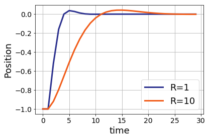
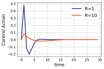
Which of these trajectories is better is a matter of the specifications given to the control engineer, and will vary on a case-by-case basis.
Takeaways
Again, I emphasize that LQR cannot capture every interesting optimal control problem, not even when the dynamics are linear. For example, the rotors can’t apply infinite forces, so some sort of constraints must be enforced on the control actions.
On the other hand, it has many of the salient features. Dynamic programming recursion lets us compute the control actions efficiently. For long time horizons, a static policy is nearly optimal. And the optimal control action can be found by minimizing a particular function which assesses future rewards. These main ideas will generalize beyond the LQR baseline. Moreover, the use of Lagrangians to compute derivatives generalizes immediately, and forms the basis of many early ideas in optimal control. Moreover, this idea also underlies Iterative LQR which solves a Taylor approximation to the optimal control problem and uses this to improve a control policy.
Now the main question to consider in the context of RL: what happens when we don’t know $A$ and $B$? What’s the right way to interact with the dynamical system in order to quickly and efficiently get it under control? The next few blogs will explore ideas from RL and how they fare when applied to this simple, linearized baseline. But first, let’s take a moment to clarify the rules of the game in contemporary Reinforcement Learning