This is the eleventh part of “An Outsider’s Tour of Reinforcement Learning.” Part 12 is here. Part 10 is here. Part 1 is here.
The essence of reinforcement learning is using past data to enhance the future manipulation of a system that dynamically evolves over time. The most common practice of reinforcement learning follows the episodic model, where a set of actions is proposed and tested on a system, a series of rewards and states are observed, and this combination of previous action and reward and state data are combined to improve the action policy. This is a rich and complex model for interacting with a system, and brings with it considerably more complexity than in standard stochastic optimization settings. What’s the right way to use all of the data that’s collected in order to improve future performance?
Methods like policy gradient, random search, nominal control, and Q-learning each transform the reinforcement learning problem into a specific oracle model and then derive their analyses using this model. In policy gradient and random search, we transform the problem into a zeroth-order optimization problem and use this formulation to improve the cost. Nominal control turns the problem into a model estimation problem. But are any of these methods more or less efficient than each other in terms of extracting the most information per sample?
In this post, I’m going to describe an iterative learning control (ILC) scheme that uses past data in an interesting way. And its roots go back to the simple PID controller we discussed in the last post.
PID control for iterative learning control
Consider the problem of getting a dynamical system to track a fixed time series. That is, we’d like to construct some control input $\mathbf{u} = [u_1,\ldots,u_N]$ so that the output of the system is as close to $\mathbf{v} = [v_1,\ldots,v_N]$ as possible (I’ll use bold letters to describe sequences). Here’s an approach that looks a lot like reinforcement learning: let’s feedback the error in our tracker to build the next control. We can define the error signal to be the difference $\mathbf{e} = [v_1-y_1, \ldots,v_n-y_N]$. Then let’s denote the discrete integral (cumulative sum) of $\mathbf{e}$ as $\mathcal{S} \mathbf{e}$. And let’s denote the discrete derivative as $\mathcal{D}\mathbf{e}$. Then we can define a PID controller over trajectories as
\[\mathbf{u}_{\mathrm{new}} = \mathbf{u}_{\mathrm{old}} + k_P \mathbf{e} + k_I \mathcal{S} \mathbf{e} + k_D \mathcal{D} \mathbf{e}\,.\]Note that these derivatives and integrals are computed on the sequence $e$, but are not a function of older iterations. In this sense, this particular scheme for ILC is different than classical PID, but it is building upon the same primitives.
This scheme is what most controls researchers think of when they hear the term “iterative learning control.” I like to take a more encompassing view of ILC, as I described in a previous post: ILC is any control design scheme where a controller is improved by repeating a task multiple times, and using previous repetitions to improve control performance. In that sense, ILC and episodic reinforcement learning are two different terms for the same problem. But the most classical example of this scheme in controls is the PID-type method I described above.
Note that this is using a ton of information about the previous trajectory to shape the next trajectory. Even though I am designing an open loop policy, I am using far more than reward information alone in constructing the policy.
How well does this work? Let’s use the simple quadrotor model we’ve been using, this time with some added friction to make it a bit more realistic. So the true dynamics will be two independent systems of the form
\[\begin{aligned} x_{t+1} &= Ax_t + Bu_t\\ y_t &= Cx_t \end{aligned}\]with
\[A = \begin{bmatrix} 1 & 1 \\ 0 & 0.9 \end{bmatrix}\,,~~ B=\begin{bmatrix} 0\\1\end{bmatrix}\,,~~\mbox{and}~~C=\begin{bmatrix} 1 & 0 \end{bmatrix}\]Let’s get this system to track a trajectory without using the model. That is, let’s use iterative learning control to learn to track some curve in space without ever knowing what the true model of the system is. To get a target trajectory, I made the following path with my mouse:
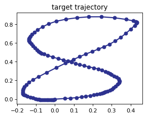
For ILC, let’s use the PID controller setup above. I’m actually only going to use the derivative term, setting $k_D = 0.1$ and the rest of the terms to $0$. Then I get the following performance for the first 8 iterations.
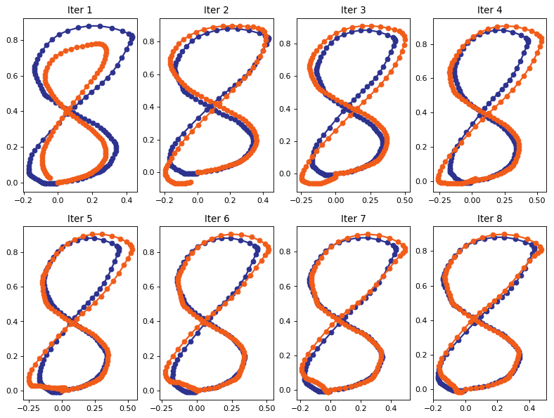
And this is what the trajectory looks like after 20 repetitions:
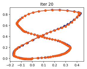
Not bad! This converges really quickly, and using all of the state information finds a control policy even without positing a model in very few iterations. Again, the update is the “D”-control update above, and this never uses any knowledge of the true dynamics that govern the system. Amazingly, there is no need for 100K episodes to get this completely model-free method to converge to a quality solution. For the curious, here’s the code to generate these plots in a python notebook
Stochastic approximation in sheep’s clothing
Why does this work? In this case, because everything is linear, we can actually analyze the ILC scheme in a simple way. Note that because the dynamics are linear, there is some matrix $\mathcal{F}$ that takes the input and produces the output. That’s what “linear” dynamics means, right?
Also, note that both $\mathcal{S}$ and $\mathcal{D}$ are linear maps so we can think of them as matrices as well. So suppose we knew in advance the optimal control input $u_\star$ such that $v=\mathcal{F} \mathbf{u}_\star$. Then, with a little bit of algebra, we can rewrite the PID iteration as
\[\mathbf{u}_{\mathrm{new}} -\mathbf{u}_\star= \left\{I +(k_P I + k_I \mathcal{S} + k_d \mathcal{D}) \mathcal{F}\right\} (\mathbf{u}_{\mathrm{old}} -\mathbf{u}_\star)\,.\]If the matrix in curly brackets has eigenvalues less than $1$, then this iteration converges linearly to the optimal control input. Indeed, with the choice of parameters I used in my examples, I actually made the update map into a contraction mapping, and this explains why the performance looks so good after 8 iterations.
This is a cute instance of stochastic approximation that does not arise from following the gradient of any cost function: we are trying to find a solution of the equation $v = F u$, and our iterative algorithm for doing so uses the classic Robbins-Monro method. But it has a very different flavor than what we typically encounter in stochastic gradients. For the experts out there, the matrix in the parentheses is lower triangular, and hence is never positive definite.
I actually think there a lot of great questions to answer even for this simple linear case: Which dynamics admit efficient ILC schemes? How robust is this method to noise? Can we use this method to solve problems more complex than trajectory tracking? It also shows that there are lots of ways to use your data in reinforcement learning, and there are far more options out there than might appear.