This is the seventh part of “An Outsider’s Tour of Reinforcement Learning.” Part 8 is here. Part 6 is here. Part 1 is here.
The role of models in reinforcement learning remains hotly debated. Model-free methods, like policy gradient, aim to solve optimal control problems only by probing the system and improving strategies based on past awards and states. Many researchers argue for systems that can innately learn without the complication of the complex details of required to simulate a physical system. They argue that it is often easier to find a policy for a task than it is to fit a general purpose model of the system dynamics.
On the other hand, in continuous control problems we always have models. The idea that we are going to build a self-driving car from trial and error is ludicrous. Fitting models, while laborious, is not out of the realm of possibilities for most systems of interest. Moreover, often times a coarse model suffices in order to plan a nearly optimal control strategy. How much can a model improve performance even when the parameters are unknown or the model doesn’t fully capture all of the system’s behavior?
In this post, I’m going to look at one of the simplest uses of a model in reinforcement learning. The strategy will be to estimate a predictive model for the dynamical process and then to use it in a dynamic programming solution to the prescribed control problem. Building a control system as if this estimated model were true is called nominal control, and the estimated model is called the nominal model. Nominal control will serve as a useful baseline algorithm for the rest of this series. In this post, let’s unpack how nominal control might work for the simple LQR problem.
System identification
Estimation of dynamical systems is called system identification in the controls community. System Identification differs from conventional estimation because one needs to carefully choose the right inputs to excite the various degrees of freedom and because dynamical outputs are correlated over time with the parameters we hope to estimate. Once data is collected, however, conventional machine learning tools are used to find the system that best agrees with the data.
Let’s return to our abstract dynamical system model
\[x_{t+1} = f(x_t,u_t,e_t)\]We want to build a predictor of $x_{t+1}$ from $(x_t,u_t,e_t)$. The question is how much do we need to model? Do we use a complicated physical model that is given by physics? Or do we approximate $f$ non-parametrically, say using a neural network? How do we fit the model to guarantee good out of sample prediction?
This question remains an issue even for linear systems. Let’s go back to the toy example I’ve been using throughout this series: the quadrotor dynamics. In the LQR post, We modeled control of a quadrotor as an LQR problem
\[\begin{array}{ll} \mbox{minimize}_{u_t,x_t} \, & \frac{1}{2}\sum_{t=0}^{N-1} x_{t+1}^TQ x_{t+1} + u_t^T R u_t \\ \mbox{subject to} & x_{t+1} = A x_t+ B u_t, \\ & \qquad \mbox{for}~t=0,1,\dotsc,N,\\ & \mbox{($x_0$ given).} \end{array}\]Where
\[\begin{aligned} A &= \begin{bmatrix} 1 & 1 \\ 0 & 1 \end{bmatrix}\, & \qquad B &= \begin{bmatrix} 0\\ 1 \end{bmatrix}\, \\ Q &= \begin{bmatrix} 1 & 0 \\ 0 & 0 \end{bmatrix}\, & \qquad R &= 1 \end{aligned}\]and we assume that $x0 = [-1,0]$.
Given such a system, what’s the right way to identify it? A simple, classic strategy is simply to inject a random probing sequence $u_t$ for control and then measure how the state responds. A model can be fit by solving the least-squares problem
\[\begin{array}{ll} \mbox{minimize}_{A,B} & \sum_{t=0}^{N-1} ||x_{t+1} - A x_t - B u_t||^2\,. \end{array}\]Let’s label the minimizers $\hat{A}$ and $\hat{B}$. These are our point estimates for the model. With such point estimates, we can solve the LQR problem
\[\begin{array}{ll} \mbox{minimize}_{u_t,x_t} \, & \frac{1}{2}\sum_{t=0}^{N-1} x_{t+1}^TQ x_{t+1} + u_t^T R u_t \\ \mbox{subject to} & x_{t+1} = \hat{A} x_t+ \hat{B} u_t, \\ & \qquad \mbox{for}~t=0,1,\dotsc,N,\\ & \mbox{($x_0$ given).} \end{array}\]In this case, we are solving the wrong problem to get our trajectory $u_t$. But you could imagine that if $(\hat{A},\hat{B})$ and $(A,B)$ are close, this should work pretty well.
Given the fact that there will be errors in the estimation, and that we don’t yet know what the right signal is to excite the different system modes, it is not clear at all how well this will work in practice. And our understanding of what is the optimal probing strategy and optimal estimation rates is still open. But it does seem like a sensible approach, and lack of theory should never stop us from trying something out…
Comparing Policies
I ran experiments for the quadrotor problem with a little bit of noise ($e_t$ zero-mean with covariance $10^{-4} I$), and with time horizon $T=10$. The input sequence I chose was Gaussian white noise with unit variance. Code for all of these experiments is in this python notebook.
With one iteration (10 samples), the nominal estimate is correct to 3 digits of precision. Not bad! And, not surprisingly, this returns a nearly optimal control policy. Right out of the box, this nominal control strategy worked pretty well. Note that I even made the nominal control’s life hard here. I used none of the sparsity information or domain knowledge. In reality, I should only have to estimate one parameter: the (2,1) entry in $B$ which governs how much force is put out by the actuator and how much mass the system has.
Now, here’s where I get to pick on model-free methods again. How do they fare on this problem? The first thing I did was restrict my attention to policies that used a static, linear gain. I did not want to wade into neural networks. This is helping the model free methods, as a static linear policy works almost as well as a time varying policy for this simple 2-state LQR problem. Moreover, there are only 2 decision variables. Just two numbers to identify. Should be a piece of cake, right?
I compared three model free strategies
-
Policy Gradient. I coded this up myself, so I’m sure it’s wrong. But I used a simple baseline subtraction heuristic to reduce variance, and also added bound constraints to ensure that PG didn’t diverge.
-
Random search. A simple random search heuristic that uses finite difference approximations across random axes.
-
Uniform sampling I picked a bunch of random controllers from a bounded cube in $\mathbb{R}^2$ and returned the one that yielded the lowest LQR cost.
How do these fare? I ran each of these methods, using 10 different random seeds, and plot the best results of 10 here:
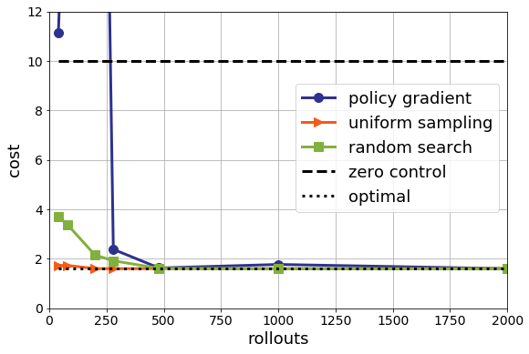
After about 500 rollouts (that is, 500 trials of length 10 with different control settings), all of the methods seem equally good. Though, again, this is comparing to one rollout for nominal control. That’s a pretty big hit to be taking in sample complexity in 2D. Random search seems to be a bit better than policy gradient, but, perhaps unsurprisingly, uniform sampling is better than both of them. It’s 2D after all.
The story changes if I include error bars. Now, rather than plotting the best performance, I plot the median performance
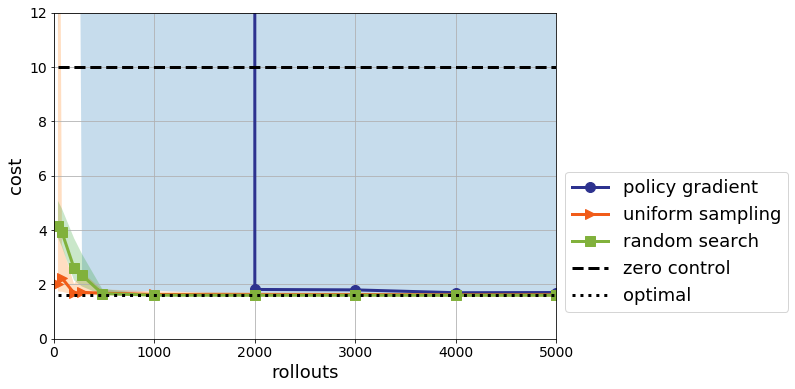
The error bars here are encompassing the max and min over all trials. Policy gradient looks much worse than it did before. And indeed, its variance is rather high. After 4000 rollouts, its median performance is on par with the nominal control with a single rollout. But note that the worst case performance is still unstable even with 5000 simulations.
My problem with policy gradients is how do I debug this? I probably have a bug! But how can I tell? What’s a unit test? What’s a simple diagnostic to know that this is working other than the fact that the cost tends to improve with more samples?
Of course, it’s probable that I didn’t tune the random seed properly to get this to work. I used 1337, as suggested by Moritz Hardt, but other values surely work better. Perhaps a better baseline would improve things? Or maybe I could add a critic? Or I could use something more sophisticated like a Trust Region method?
All of these questions are asking for more algorithmic complexity and are missing the forest for the trees. The major issue is model-free methods are several orders of magnitude worse than a parameter-free, model-based method. If you have models, you really should use them!
MetaLearning
Another claim frequently made in RL is that policies learned in one task may generalize to other tasks. A rather simple form of generalization would be to be able to achieve high performance on the LQR problem as we change the time horizon. That is, what if we make the length of the horizon arbitrarily long, will the policies still achieve high performance?
One way to check this would be to see what the cost looks like on an infinite time horizon. If we do nominal control, we can plug in our point estimate and solve a Ricatti equation and produce a controller for an infinite time horizon. As expected, this is nearly optimal for the quadrotor model.
But what about for the model-free approaches? Do the learned controllers generalize to arbitrarily long horizons? With model-free methods, we are stuck with a fixed controller, but can test it on the infinite time horizon regardless. The results look like this:
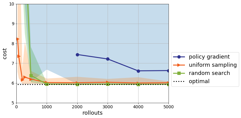
The error bars for Policy Gradient are all over the place here, and the median is indeed infinite up to 2000 rollouts. What is happening is that on an infinite time horizon, it is necessary for the controller to be stabilizing so that the trajectories don’t blow up. A necessary and sufficient condition for stabilization is for the matrix $A+BK$ to have all of its eigenvalues to be less than 1. This makes sense, as the closed-loop system takes the form
\[x_{t+1} = (A+BK)x_t + e_t\]If $A+BK$ has an eigenvalue with magnitude greater than 1, then that corresponding eigenvector will be amplified exponentially quickly. We can plot how frequently the various search methods find stabilizing control policies when looking at a finite horizon. Recall that nominal control finds such a policy with one simulation.
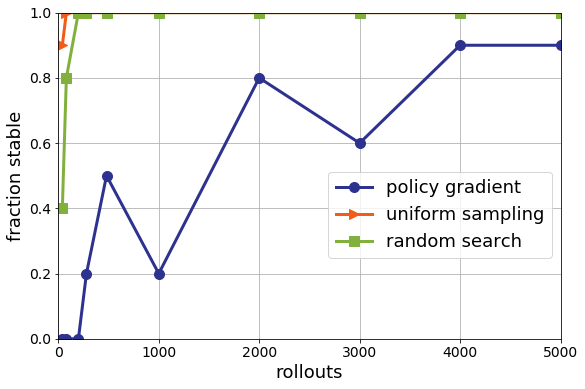
Uniform sampling and random search do eventually tend to only find stabilizing policies, but that they still require a few hundred simulations to ensure stability. Policy gradient, on the other hand, never returns a stabilizing policy more than 90 percent of the time, even after thousands of simulations.
A Coarse Model Can’t Do Everything
Though I expect that a well-calibrated coarse model will outperform a model-free method on almost any task, I want to close by emphasize that we do not know the limits of model-based RL any more than we know the limits of model-free. Even understanding the complexity of estimation of linear, time-invariant systems remains an open theoretical challenge. In the nonlinear case, affairs are only harder. We don’t fully understand the limits and fragilities of nominal control for LQR, and we don’t know just how coarse of a model is needed to attain satisfactory control performance. In future posts, I will address some of these limits and the open problems we’ll need to solve in order make learning a first-class citizen in contemporary control systems.